Automotive manufacturing
Allocating scarce production capacity across a North American vehicle lineup
Mixed-integer optimization that allocated constrained production capacity across about 200 vehicle types and a 24-month horizon, balancing profit, volume, and emissions.
$390M
Project-reported incremental profit estimate
40,000
Additional vehicles per year, project-reported
Client
Global automotive manufacturer
Basis
Partner experience, prior role
The insight
“A vehicle mix that looks attractive in isolation may block a more valuable combination elsewhere in the network. Neither a demand ranking nor a unit-margin ranking finds the best feasible mix.”
Exhibit
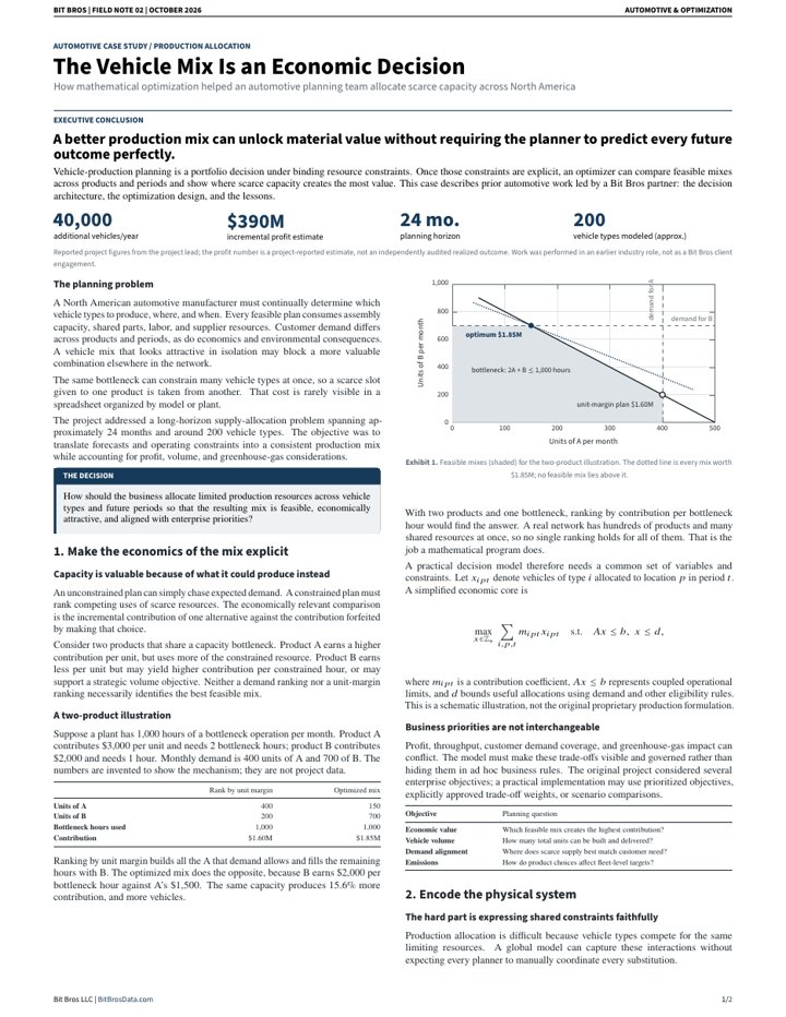
Ranking by unit margin leaves 15.6% on the table
Feasible monthly mixes of two products sharing one bottleneck
Illustrative, from Field Note 02: 1,000 bottleneck hours; product A earns $3,000 and uses 2 hours, product B earns $2,000 and uses 1; demand is 400 A and 700 B. B earns more per bottleneck hour, so the optimum builds all the B demand allows.
Which vehicles to build, where, and when
A North American automotive manufacturer must continually decide which vehicle types to produce, where, and when. Every plan consumes assembly capacity, shared parts, labor, and supplier resources, and demand, economics, and emissions differ across products and periods. The work covered a supply-allocation problem spanning about 24 months and around 200 vehicle types.
One bottleneck constrains many products at once
The same scarce component or production slot can serve many vehicle types, so giving it to one product takes it from another. That cost is rarely visible in a spreadsheet organized by model or plant, and a local improvement in one place can make the network worse elsewhere. Profit, volume, demand coverage, and greenhouse-gas targets also pull in different directions.
A global allocation model the planners could govern
We formulated a mixed-integer optimization model that allocated constrained production across vehicle types, plants, and periods, with plant capacity, shared components, product eligibility, demand and mix bounds, multi-period balance, and environmental limits modeled together. Rules that were physics stayed hard; preferences became explicit trade-offs.
The planner workflow was treated as part of the model: versioned forecasts and assumptions, explained infeasibilities, scenario comparison before approval, and attention to plan stability so small input changes did not trigger disruptive swings.
Value from a better feasible mix
The project lead reported about 40,000 additional vehicles per year and an incremental profit estimate of about $390 million against the planning baseline. These are project-reported figures, not independently audited realized outcomes. The mechanism is a better feasible mix: even with fixed capacity, economic output changes when the allocation of that capacity changes.
Field Note 02 / 2-page PDF
The Vehicle Mix Is an Economic Decision
The full write-up: the planning problem, a worked two-product example, the constraint families, the planner workflow, what the project reported, and lessons that transfer beyond automotive.
What made the difference
01
Make the economics explicit
Every scarce build slot was valued by the contribution it could earn elsewhere, so each exception carried a visible opportunity cost.
02
Encode the shared constraints
Plant capacity, shared components, eligibility, demand bounds, and emissions limits were modeled together, so one global plan replaced many local ones.
03
Design for the planner
Versioned inputs, explained infeasibilities, scenario comparison, and change penalties kept a long-horizon plan stable and reviewable.