Flagship guide / Decision Science
The Sequential Decision Toolbelt
How to choose the right policy, model, and algorithm
From Powell's four policy classes to practical engineering decisions: a guide to what to use, when to use it, and why.
Adam DeJans Jr. | | Interactive reference, 71 methods
The argument in brief
Choosing a policy is an engineering decision, and it can be made deliberately.
The literature on sequential decisions is vast. Mathematical programming, stochastic optimization, approximate dynamic programming, simulation, and reinforcement learning each have deep textbooks and decades of results. What that literature rarely answers is the question a practitioner actually faces on a Monday morning: given this plant, these data, and this decision cadence, what should we build first, what should we compare it against, and how will we know whether it works?
This guide answers that question with a framework rather than a catalog. It rests on Warren B. Powell's observation that every method for making sequential decisions belongs to one of four classes of policies, or to a hybrid of them (Powell, policies). We add a practitioner layer on top: a strict separation between a policy's architecture and the algorithms that implement or tune it, a method library of 71 techniques cross-referenced to the classes they can serve, an advisor that turns problem structure into testable hypotheses, and a worked manufacturing example in which every number comes from code that runs.
Three principles carry the argument. First, keep the layers apart: the decision problem, the policy architecture, the mathematical engine, the tuning mechanism, and the validation process are different things, and most confused projects confuse two of them. Second, start with the simplest credible policy and add sophistication only when the structure and economics of the problem justify it. Third, judge every policy by its performance over simulated or replayed trajectories, out of sample, because that is the only place where policies of different classes can be compared on equal terms.
The worked example makes the second principle concrete, and the result is less flattering to sophistication than many teams expect. On our illustrative three-family production line, tuning a two-parameter rule recovered 83% of the savings achieved by the best policy we built, and an untuned deterministic lookahead did no better than that tuned rule. The four strongest policies, spanning three classes and two hybrids, were separated by only 2.2% of the baseline's cost. On this problem, the decisive steps were writing down the economics, tuning against them, and evaluating honestly; the choice among sophisticated classes mattered less. Your problem will differ, which is precisely why the evaluation discipline matters more than any single recommendation.
New to the four classes
Read sections 1 to 3, then explore the taxonomy.
Start with the classes →Have a problem in hand
Answer eight questions, then check the method matrix and the hybrids.
Go to the advisor →Already built a policy
Read sections 7 and 9 on tuning, evaluation, and what the numbers do and do not show.
Tuning and evaluation →At a glance
The toolbelt on one page
Everything in this guide in a single picture: the model you build once, the four policy classes with the conditions that favor each, the methods and software behind them, and the loop that tunes, evaluates, and deploys the result.
Exhibit
The Toolbelt on one page
Model the problem once, choose a policy architecture, then tune and evaluate it. Software listed is representative, not exhaustive.
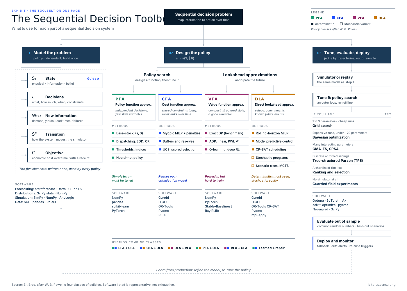
1 · Model the problem
policy-independent; build once
- Sₜ StateGuide →physical · information · belief
- aₜ Decisionswhat, how much, when; constraints
- Wₜ₊₁ New informationdemand, yields, lead times, failures
- Sᴹ Transitionhow the system moves: the simulator
- C Objectiveeconomic cost over time, with a receipt
Forecasting: statsforecast · Darts · GluonTS
Distributions: SciPy.stats · NumPy
Simulation: SimPy · NumPy · AnyLogic
Data: SQL · pandas · Polars
2 · Design the policy
aₜ = π(Sₜ | θ)
Policy search · design a function, then tune it
PFA Policy function approx.
When: independent decisions, few state variables
Base-stock, (s, S) · Dispatching: EDD, CR · Thresholds, indices · Neural-net policy
Simple to run, must be tuned
Software: NumPy · pandas · scikit-learn · PyTorch
CFA Cost function approx.
When: shared constraints today, weak links over time
Myopic MILP + penalties · Buffers and reserves · UCB, scored selection
Reuses your optimization model
Software: Gurobi · HiGHS · OR-Tools · Pyomo · PuLP
Lookahead approximations · anticipate the future
VFA Value function approx.
When: compact, structured state, a good simulator
Exact DP (benchmark) · ADP: linear, PWL V̄ · Q-learning, deep RL
Powerful, but hard to train
Software: NumPy · PyTorch · Stable-Baselines3 · Ray RLlib
DLA Direct lookahead approx.
When: setups, commitments, known future events
Rolling-horizon MILP · Model predictive control · CP-SAT scheduling · Stochastic programs (stochastic) · Scenario trees, MCTS (stochastic)
Deterministic: most used; stochastic: costly
Software: Gurobi · HiGHS · OR-Tools CP-SAT · Pyomo · mpi-sppy
Hybrids: PFA + CFA · CFA + DLA · DLA + VFA · PFA + DLA · VFA + CFA · Learned + repair
3 · Tune, evaluate, deploy
judge by trajectories, out of sample
- Simulator or replaythe same model as step 1
- Tune θ: policy search
- 1 to 3 parameters, cheap runs → Grid search
- Expensive runs, under ~20 parameters → Bayesian optimization
- Many interacting parameters → CMA-ES, SPSA
- Discrete or mixed settings → Tree-structured Parzen (TPE)
- A shortlist of finalists → Ranking and selection
- No simulator at all → Guarded field experiments
Software: Optuna · BoTorch · Ax · scikit-optimize · pycma · Nevergrad · SciPy
- Evaluate out of samplecommon random numbers · held-out scenarios
- Deploy and monitorfallback · drift alerts · re-tune triggers
↺ Learn from production: refine the model, re-tune the policy
The map reads top to bottom, but the work does not. The three parts hand information back and forth in loops that run at very different speeds. The design loop between policy and tuning turns over in hours. The validation loop, triggered when a simulator cannot reproduce history, sends the team back to the model, and usually reveals a missing state variable or a cost nobody wrote down. The operating loop runs for the life of the system: production exposes drift, overrides, and late data that no design session anticipated, and each of them should change the model or the tuning, not just the planners' workarounds.
Exhibit
How the three parts interact: one lifecycle, three loops
Numbered arrows are handoffs. Color marks the loop each belongs to; the loops run at very different speeds.
- 01 Model → policy: defines what a policy may read, decide, and optimize
- 02 Policy → tuning: candidate class and parameters θ
- 03 Tuning → policy: tuned θ, or evidence to change class
- 04 Tuning → model: simulation disagrees with history: missing state, wrong costs
- 05 Tuning → production: validated policy, fallback, thresholds
- 06 Production → model: drift, overrides, late data, new constraints
- 07 Production → tuning: re-tune triggers
Design loop
Steps 02, 03 · offline · hours to days
Propose a policy architecture and parameters, simulate, compare, repeat. Most of the engineering effort lives here.
Validation loop
Steps 04 · weeks
When the simulator cannot reproduce history, the fault is in the model, not the policy. Fix the state, the costs, or the uncertainty model, then return to design.
Operating loop
Steps 05, 06, 07 · months, continuously
Deploy with a fallback, watch for drift and overrides, re-tune when thresholds trip, and feed what production teaches back into the model.
Part 1
Decisions are functions of state
A sequential decision system maps information into actions, repeatedly, as new information arrives. The object we design is therefore not a plan, which is a list of numbers, but a policy, which is a rule for producing numbers in any situation, including situations no plan anticipated. We write it as
where is the state at time , the action, the structure of the policy, and its tunable parameters. Powell writes the same object as ; the notation differs, the idea does not. A complete model of the problem has five elements, which Powell's universal modeling framework makes explicit (Powell, universal modeling framework). We introduce them through the example that runs through this guide.
Line 3 is a single production line making three product families, A, B, and C. Each week the planner decides which families to set up and how many units of each to make. Changeovers consume line time and money, at most two are allowed per week, production released this week serves next week's demand, demand is seasonal and uncertain, and demand that cannot be served is lost.
- State . Everything needed to decide, and nothing more: the inventory of each family at the end of week and the week of the season, which determines the forecast. In a real plant it would also include work in process, open orders, and machine status. Getting the state right is a design problem in its own right, covered in our companion guide The State Variable (see also Inventory position is a state, not a number).
- Action . Which families to set up and the quantity of each, subject to line capacity and the changeover limit.
- Exogenous information . What the world reveals after the decision: next week's demand for each family.
- Transition . Inventory carried forward is what was available minus what was sold: .
- Objective. Minimize expected total cost over the horizon, the sum of changeover, holding, and lost-sales costs, across the policies we are willing to consider:
Two features of this objective deserve emphasis because they drive everything that follows. The expectation is taken over trajectories: a policy is judged by what happens when it is applied week after week to an uncertain future, not by the quality of any single decision. And the minimization is over policies, a space of functions, which is why the practical questions are which family of functions to search and how to search it.
Exhibit
Line 3: three families, one line, one seasonal peak
Expected weekly demand across the 13-week season, against line capacity
Week of season · amber weeks exceed what two changeovers leave
| Family | Base / wk | Hold / unit | Short / unit |
|---|---|---|---|
| A | 30 | 1 | 10 |
| B | 18 | 1.2 | 14 |
| C | 12 | 1.5 | 18 |
Base demand totals 60 units a week. In the peak it reaches 102, so the line must build ahead. Changeovers make small, frequent runs expensive, and running all three families every week is not allowed.
Illustrative model used throughout this guide. Capacity is 90 units of line time per week; each changeover consumes 10 units and costs 120; at most 2 changeovers per week. Weekly demand is lognormal around the seasonal mean with a coefficient of variation of 0.35. Production released this week serves next week's demand; unmet demand is lost.
Part 2
Five layers, not one
Most confused decision projects fail by mixing two of these layers. Name them separately and many arguments dissolve.
The decision problem and the physical system
What is decided, when, with what information, at what cost, under which constraints?
Line 3Three families, 90 units of line time, changeovers, lost sales, seasonal demand.
Not a model yet. It is the reality the model must respect.
The policy architecture
How does a state become an action: a rule, a tuned optimization, a learned value, or an explicit lookahead?
Line 3A three-week rolling-horizon lookahead with a tuned demand buffer (CFA + DLA).
This is the only layer where PFA, CFA, VFA, and DLA live.
The mathematical representation and algorithms
How is the policy's computation expressed and solved?
Line 3Setup patterns enumerated, each quantity problem solved as a min-cost flow. A plant-scale version would be a MILP solved with Gurobi, HiGHS, or CP-SAT.
Solvers and formulations implement a policy. They are not policies.
The tuning or improvement mechanism
How are the policy's parameters or functions chosen?
Line 3Grid search over 9 buffer values on 40 training scenarios.
Bayesian optimization, CMA-ES, or ADP improve a policy of any class.
Simulation, validation, and deployment
How do we know it works, and what happens when it does not?
Line 3100 held-out test years with common random numbers; in production, replay, monitoring, and a fallback rule.
A simulator evaluates decisions. It does not make them.
Six category errors, corrected
The layers sound obvious when listed. In practice they blur, usually because a tool's name becomes shorthand for the whole system. The table below lists statements we hear regularly and where each component actually belongs.
| What gets said | Layer | What is actually true |
|---|---|---|
| "Our policy is Gurobi." | 3 | Gurobi is a solver. It can implement the optimization inside a CFA, a VFA, or a DLA. The policy is the model it solves, how that model is parameterized, and how often it is re-solved. |
| "We use Bayesian optimization as our policy." | 4 | Bayesian optimization tunes parameters. It can tune the reorder points of a PFA, the penalties of a CFA, or the buffer of a DLA. It never makes the weekly decision itself. |
| "The probabilistic forecast solves it." | 1, 3 | A probabilistic forecast is information about uncertainty. Every class can consume it, and every class still needs a rule for turning it into an action (see From distribution to decision). |
| "We are doing RL instead of optimization." | 2, 4 | Reinforcement learning algorithms produce policies in the four classes: policy-gradient methods produce PFAs, Q-learning produces VFAs, and model-based RL plans with a lookahead. The useful questions are which class and how it is trained. |
| "The digital twin will make the decisions." | 5 | A simulator evaluates a policy over sampled futures. It is indispensable for tuning and comparison, but something still has to choose the action (see A simulator is not a policy). |
| "The MILP is optimal, so the policy is optimal." | 2, 3 | A proven optimal solution is optimal for one model of one period or horizon. Whether repeatedly solving that model yields good performance over time is a separate, empirical question (see The MIP gap is a decision bound). |
Part 2, continued
Model first, policy second
Powell's universal modeling framework separates two activities that most projects fuse: modeling the problem and designing the policy. The model is the five elements of Part 1, the state, the decisions, the exogenous information, the transition function, and the objective. It describes the physics, the information, and the economics, and it is written down before any policy is chosen. The policy is then a function that plugs into the model, one candidate among many. Powell stresses that modeling the problem, and in particular identifying the decisions, deserves more attention than the hunt for the best-performing policy usually leaves it.
Keeping the two apart has three practical consequences.
- Every candidate is judged on the same terms. The objective, the transitions, and the uncertainty do not change when the policy changes. That is the only reason the eight Line 3 policies in Part 9, from a hand-set rule to a learned hybrid, can be compared at all: one model, one simulator, one cost accounting, eight plug-ins.
- A policy's internal model is not the model. A CFA's tuned penalties and a DLA's point-forecast lookahead are approximations that live inside the policy; the tildes in the DLA formula of Part 3 mark exactly this. They can be deliberately wrong while the base model stays right. Teams that fuse the two end up "correcting" the business objective when they should be tuning the policy (see Cost functions are policy knobs).
- The software follows the separation. Build the model and simulator with a narrow policy interface, a function from state to action, so that policies can be swapped, benchmarked, and replaced without touching the physics or the economics. The production system calls the same interface.
One qualification keeps the separation honest. Because the state is whatever the decision, costs, and transitions need, choosing a policy can add to the information state: a lookahead needs forecasts that a reorder-point rule does not. That adds inputs to the model; it never changes the physics or the objective. The companion guide, The State Variable, develops this in detail.
The model · fixed
- State:
- inventory by family, week of season
- Decisions:
- setups and quantities, at most two runs
- Information:
- next week's demand
- Transition:
- carry forward what was not sold
- Objective:
- changeover + holding + lost sales
← at
The policy · interchangeable
- Hand-set rule
- Tuned PFA
- Tuned CFA
- Deterministic DLA
- Buffered DLA
- Myopic expected cost
- VFA (trained by ADP)
- DLA + VFA
The eight Line 3 policies from Part 9, all evaluated in the same model.
Part 3
The four classes of policies
Powell's framework, with full credit: four meta-classes that, in his words, span any method for making decisions. Two strategies group them.
Powell divides policies into two broad strategies. Policy search designs a function that does not plan into the future explicitly and tunes it to perform well over time; it contains the PFA and the CFA. Lookahead approximations estimate the downstream consequences of today's decision; they contain the VFA, which approximates the value of the state a decision leads to, and the DLA, which optimizes over an explicit model of the future. Powell observes that PFAs, CFAs, and deterministic DLAs dominate practice, that VFAs have attracted the most academic attention, and that the best advice is to begin with the simplest policy that makes sense for the application, accepting that the price of simplicity is tunable parameters and that tuning is hard (Powell, policies).
No class is universally superior. In Powell's energy-storage experiments, each of several policies was the best performer on at least one variation of the same problem. The class that fits depends on coupling, intertemporal structure, the role of uncertainty, the shape of the state, the decision cadence, and the data, which is why the advisor in Part 5 asks about exactly those things.
Strategy: Policy search
Functions that do not plan into the future explicitly. They are designed and then tuned, by simulation or field experience, to perform well over time.
Strategy: Lookahead approximations
Policies that estimate the downstream consequences of today's decision, either through an approximate value of the resulting state or through an explicit model of the future.
| PFA | CFA | VFA | DLA | |
|---|---|---|---|---|
| Solved at decision time | Nothing: evaluate a function | A modified one-period model | Immediate cost plus approximate value | A model of the next H periods |
| How the future enters | Through the rule's shape and tuning | Through tuned penalties and buffers | Through a learned value of the resulting state | Explicitly, as a forecast or scenarios |
| What is tuned or learned | Rule parameters | Penalties, bonuses, buffers | Value function parameters | Horizon, buffers, scenario set |
| Typical engine | None, or a lookup | LP, MILP, assignment | LP or MILP with value terms | MILP, CP-SAT, stochastic programs |
| Main risk | Blind to coupling | Penalties summarize the future crudely | Unreliable value estimates | Ignores risk if deterministic; costly if not |
Class 1 / Policy search
Policy function approximation (PFA)
A rule that maps the state directly to a decision.
A PFA is an explicit function from the state to an action. Nothing is optimized when the decision is made: the rule is evaluated and the action follows. All of the intelligence lives in the functional form, chosen by the designer, and in its parameters, chosen by tuning. Powell notes that this is the only one of the four classes that does not solve an embedded optimization problem.
An order-up-to rule: R_t is inventory position and θ^S the target. The parameter vector θ is the policy's only lever.
On Line 3, the worked example
On Line 3 a PFA sets each family's target as a multiple of its average forecast over the next three weeks, runs a family only if its shortfall is large enough to justify a changeover, and serves at most two families per week in order of shortage cost times shortfall. Two numbers, the cover multiple and the minimum run size, are tuned by simulation.
- Common implementations
- Order-up-to and (s, S) inventory rules, dispatching rules such as EDD and critical ratio, condition-based maintenance thresholds, weighted priority indices, lookup tables, affine decision rules, and neural networks trained to output actions.
- Data requirements
- The state variables the rule reads, plus a simulator or historical replay to tune the parameters. Because tuning evaluates performance directly, a PFA never needs an explicit model of costs inside the rule.
- Computational and implementation tradeoffs
- Nearly free to execute and easy to audit, but every structural insight must be designed into the functional form. Parameters multiply quickly when a rule is indexed by item, season, or regime, and tuning becomes the main cost.
- Strengths
- Microsecond decisions, suitable for the shop floor and for very large item counts
- Transparent and easy to override, which builds trust with planners
- Provably optimal forms exist for several classical problems
- Naturally robust: few parameters, little to go wrong
- Weaknesses
- Cannot see coupling constraints unless rationing logic is written in by hand
- Does not anticipate known future events unless the rule is indexed on them
- Tuning many parameters is hard, and tuned values drift as conditions change
- Conditions that favor it
- Decisions that are mostly independent across items, a state that is low-dimensional or well summarized by a few features, tight latency, and a known structural result to start from.
- Warning signs
- Planners repeatedly override the rule in the same situations; parameters are re-tuned constantly; the rule's recommendations collectively violate a shared capacity, budget, or truck limit; one parameter set cannot fit both the peak and the quiet season.
- If it underperforms, try next
- If the failures are due to coupling, wrap the rule's targets in a small optimization (PFA + CFA). If they are due to anticipating known events, try a rolling-horizon lookahead. If parameters are simply many, change the tuning method before changing the class.
Class 2 / Policy search
Cost function approximation (CFA)
A deterministic optimization, parameterized and tuned to perform well over time.
A CFA solves an optimization problem at each decision, but the problem is a deliberately modified version of the immediate one: some costs are replaced by tunable penalties or bonuses, some constraints by tunable buffers. The modifications are not accounting truths; they are policy parameters chosen because the resulting sequence of decisions performs well over time.
The modified cost C̄ and the modified feasible region A_t(θ) are where the tuning happens. With θ set to its literal values the policy is simply myopic.
On Line 3, the worked example
On Line 3 a CFA solves a one-week model: choose setups and quantities to minimize setup cost plus a shortage penalty on any shortfall against an inflated requirement and a holding cost above it. Three parameters are tuned: how many weeks of forecast the requirement covers, a percentage buffer on that requirement, and a multiplier on the setup cost. The model is solved exactly each week.
- Common implementations
- Myopic LPs and MILPs with tuned penalties, capacity allocation with tunable opportunity costs, soft constraints with tuned slack penalties, assignment models with parameterized scores, upper confidence bound selection, and buffers or reserves inside deterministic models.
- Data requirements
- Everything the deterministic model needs (capacities, costs, forecasts) plus a simulator or replay set for tuning. The quality of the tuning set matters as much as the model.
- Computational and implementation tradeoffs
- Handles coupling and constraints that rules cannot, at the cost of an optimization per decision. The parameters are few and interpretable, but each tuning evaluation now runs many solves.
- Strengths
- Respects shared constraints exactly at each decision
- Reuses an existing deterministic model; often the cheapest upgrade available
- Penalties are explainable as economic levers
- Among the most widely used policies in practice
- Weaknesses
- Sees the future only through what the penalties summarize
- Literal costs make it myopic; tuned costs can hide poor modeling
- Tuning several interacting penalties requires a disciplined search
- Conditions that favor it
- Decisions coupled through shared resources today, with intertemporal effects that are real but can be summarized by a few penalties, bonuses, or buffers.
- Warning signs
- The best penalty changes with the season; the model keeps making decisions that are cheap today and expensive next month in recognizable patterns; planners add hard rules to stop specific failures; tuned penalties hit the edges of their search range.
- If it underperforms, try next
- If the failures are tied to identifiable future events, extend the model across a horizon (CFA + DLA). If they are tied to the value of carrying resources forward, learn that value (VFA + CFA).
Class 3 / Lookahead approximation
Value function approximation (VFA)
Today's cost plus an approximate value of where the decision leaves you.
A VFA chooses the action that minimizes the immediate cost plus an approximation of the expected cost from the resulting state onward. It is built on Bellman's equation. Exact dynamic programming computes that downstream value precisely; a VFA approximates it, because for realistic state spaces the exact value function cannot be computed or stored.
S^a_t is the post-decision state: where the system stands after the decision and before new information arrives. V̄_t approximates the expected cost from there on.
On Line 3, the worked example
On Line 3 a VFA solves the same one-week problem as the CFA but replaces the tuned penalties with two terms: the exact expected cost of next week's holding and shortage, computed from the demand distribution, and a learned convex value of the units carried beyond next week, one piecewise-linear curve per family and season phase. The curves are learned by approximate dynamic programming from sampled marginal values.
- Common implementations
- Bellman-based decision rules with linear, piecewise-linear, or neural value approximations; approximate dynamic programming with post-decision states; fitted value iteration; temporal-difference learning; approximate Q functions; learned terminal values.
- Data requirements
- A simulator or transition model good enough to generate experience, and a value approximation architecture that matches the problem's structure. Historical decisions are not required, but historical states help initialize.
- Computational and implementation tradeoffs
- Can capture long-run effects that no horizon of practical length covers, at the price of a difficult offline learning problem. When the approximation is linear or concave and separable, decisions remain fast optimization problems.
- Strengths
- Captures the value of carrying resources forward without an explicit long horizon
- Fast decisions once trained
- Exploits structure such as concavity in resource levels
- Exact DP on small versions provides benchmarks for every other class
- Weaknesses
- Training is delicate: step sizes, exploration, and approximation design all matter
- The curse of dimensionality returns if the approximation must capture interactions
- An unreliable value approximation produces confident, systematic errors
- Conditions that favor it
- Resource allocation problems with many interchangeable units, recurring dynamics, and structure (separability, concavity) that a simple approximation can exploit; problems where the relevant future is long relative to any affordable horizon.
- Warning signs
- Learned values oscillate or depend on the random seed; performance is good in training and poor out of sample; the policy behaves strangely in states rarely visited during training; the team cannot explain why a value has the shape it has.
- If it underperforms, try next
- If the value is unreliable, shorten its job: use it only as a terminal value at the end of a lookahead (DLA + VFA), or replace it with tuned penalties (CFA). If interactions dominate, consider a deterministic lookahead that represents them explicitly.
Class 4 / Lookahead approximation
Direct lookahead approximation (DLA)
Optimize over an explicit model of the future, implement the first decision, repeat.
A DLA solves an approximate model of the future over a planning horizon and implements only the decision for now. The lookahead model can be deterministic (point forecasts), stochastic (scenarios, trees, recourse), or robust. Its simplifications (horizon length, aggregation, how uncertainty is represented) are themselves design choices that should be tested by simulating the policy.
Tildes mark the lookahead model, an approximation of the real one. A deterministic lookahead replaces the expectations with point forecasts and optimizes a plan; a stochastic lookahead keeps them, usually through scenarios.
On Line 3, the worked example
On Line 3 a deterministic DLA plans three weeks at a time: it chooses setups and quantities for this week and the next two, using point forecasts, and implements only this week's run. It is solved exactly by enumerating setup combinations and solving a min-cost flow for each. A tuned variant inflates the forecasts by a buffer, which makes it Powell's parameterized deterministic lookahead.
- Common implementations
- Rolling-horizon deterministic optimization, model predictive control, multi-period MILPs, CP-SAT lookahead scheduling, two-stage and multistage stochastic programs, scenario trees, sample-average lookaheads, robust and chance-constrained lookaheads, and rollout or Monte Carlo tree search.
- Data requirements
- Forecasts over the horizon (and, for stochastic lookaheads, joint scenarios), plus every constraint and cost the plan must respect. The data burden is the highest of the four classes.
- Computational and implementation tradeoffs
- Handles complex, time-varying, constrained problems with no training phase, which is why it is the workhorse of industrial planning. The price is solve time per decision, and, for stochastic versions, scenario modeling effort and model size.
- Strengths
- Anticipates known future events: peaks, outages, promotions, contract dates
- Needs no training; adapts immediately when data change
- Represents rich constraints and multi-period logic
- Deterministic versions are familiar to planners and easy to explain
- Weaknesses
- A deterministic lookahead treats forecasts as certain and does not hedge
- Horizon truncation produces end effects without a terminal value
- Stochastic versions are expensive to build, solve, and validate
- Conditions that favor it
- Strong intertemporal coupling (setups, build-ahead, lead times, commitments), non-stationary forecasts, and time to solve an optimization at each decision.
- Warning signs
- The plan changes drastically from one run to the next (nervousness); inventory is run down toward the end of every horizon; a longer horizon makes performance worse; adding scenarios changes the first decision a lot.
- If it underperforms, try next
- If the lookahead ignores risk, first tune buffers (CFA + DLA), then test a stochastic lookahead against the tuned deterministic one. If end effects dominate, add a terminal value (DLA + VFA). If solves are too slow, use a rule for routine states (PFA + DLA) or decompose.
Exact results and approximations
It helps to be precise about what is proven and what is engineering judgment. Some PFAs are provably optimal for specific models: base-stock for a single item with linear costs and backlogging, (s, S) when a fixed ordering cost is added (Scarf, 1960), earliest due date for maximum lateness on one machine. Exact dynamic programming is optimal for the model it solves, whenever it can be solved at all. Everything else in this guide is an approximation: CFAs approximate the future with penalties, VFAs with a learned function, DLAs with a truncated and simplified model of the future. That is not a weakness to apologize for. Real problems violate the assumptions behind every optimality result, so the relevant comparison is always between approximations, and it is settled by simulation, not by the elegance of the method (see Dynamic programming is a policy language, not a silver bullet).
A related distinction separates explicit lookahead from approximate downstream value. A DLA represents the future as decisions and events in a model; a VFA compresses everything after the decision into a function of the post-decision state. The first is transparent and data-hungry; the second is compact and only as good as its training. Combining them, as Part 8 shows, is often the best of both.
Part 4
The interactive taxonomy
Policy architecture on top, implementation techniques below. Select any node to inspect it; hybrids and shared techniques light up every class they touch.
Sequential decision policies
Policy search
Lookahead approximations
Hybrids connect classes
PFA / Policy function approximation
CFA / Cost function approximation
VFA / Value function approximation
DLA / Direct lookahead approximation
Implementation techniques: not policy classes
Select a technique to see which classes it can serve. A solver, a forecast, or a tuning method can sit inside several architectures; none belongs to exactly one.
Decision engines · Solvers and algorithms that compute a decision inside a CFA, VFA, or DLA.
Uncertainty representation · Descriptions of what might happen. Every class consumes them.
Policy search and tuning · Outer-loop optimizers that adjust θ for any class.
Learning methods · Fit values, actions, or forecasts from data or simulation.
The tree follows Powell's two strategies and four classes; the families, the placement of methods, and the cross-references are our own synthesis for practitioners. Methods appear under a class when they are a way of building that class. A technique that serves several classes appears in the lower band instead, so that no solver, forecast, or tuning method is presented as belonging to exactly one architecture.
Part 5
Which policy should I try?
Eight questions about the structure of your problem, three kinds of answer: a practical starting policy, credible alternatives to compare against, and the conditions under which to escalate.
The advisor encodes engineering heuristics, not theorems. It favors the simplest credible policy that respects the structure you describe, names the alternatives a careful team would test it against, and states the evidence that should trigger something more sophisticated. Each recommendation shows the reasoning that produced it, so you can disagree with a specific step rather than with a verdict. Start from one of the examples, then change the answers to match your own problem.
These are engineering hypotheses to test on your own scenarios, not a guaranteed optimal choice. There is no universally correct decision tree for policy selection; the rules are written out in the page source so you can disagree with any step.
Reference chart
Which policy to try first
The advisor's logic as a single reference chart. Every path ends in a starting policy and what to compare it against.
Is the decision repeated, with new information arriving between decisions?
No, made essentially once
A single stochastic optimization, not a policy design problem
- Methods:
- Two-stage stochastic program; sample average approximation; robust optimization if the distribution is doubtful
- Engines:
- LP, MILP, Benders decomposition
- Software:
- Gurobi, HiGHS, Pyomo, mpi-sppy
- Compare:
- Deterministic model plus scenario stress tests
Yes
Are decisions coupled through shared capacity, budgets, or crews today?
No, items can be decided one at a time
Do setups, lead times, or seasonality link periods strongly?
No
Tuned inventory rule
- Methods:
- Base-stock or order-up-to; newsvendor quantile from a probabilistic forecast
- Engines:
- None at decision time; closed form or simulation offline
- Tune with:
- Grid search with common random numbers
- Software:
- NumPy, SciPy, statsforecast
Yes
Rule with forecast-indexed parameters
- Methods:
- (s, S) with seasonal or forecast-indexed targets; minimum run sizes
- Engines:
- Wagner-Whitin dynamic programming for a per-item benchmark
- Tune with:
- Coordinate search or Bayesian optimization
- Compare:
- Per-item rolling-horizon lookahead (DLA)
Yes
How much time per decision, and how strongly does today constrain tomorrow?
Milliseconds
Priority rule, optimization in the background
- Methods:
- Dispatching rules (EDD, critical ratio, ATC); weighted priority index; rule for routine states, asynchronous lookahead for hard ones
- Engines:
- None online; CP-SAT or MILP offline or asynchronously
- Tune with:
- CMA-ES or Bayesian optimization on the weights
- Escalate:
- Learned proposal plus optimization repair, if a faithful simulator exists
Seconds or more; weak links over time
Myopic optimization with tuned penalties
- Methods:
- LP or MILP of the current period with tuned shortage, slack, and opportunity-cost terms
- Engines:
- LP, MILP, assignment
- Tune with:
- Grid search or Bayesian optimization on the penalties
- Software:
- Gurobi, HiGHS, OR-Tools, Pyomo, PuLP
Seconds or more; inventory or backlog carries forward
Optimization that prices what is carried forward
- Methods:
- Tuned ending-inventory terms (CFA); separable piecewise-linear value of carried resources learned by ADP (VFA + CFA)
- Engines:
- LP or MILP with value terms
- Tune with:
- Bayesian optimization; ADP training for the value function
- Software:
- Gurobi, HiGHS, Pyomo, NumPy, PyTorch
Seconds or more; setups, commitments, or known events
Does uncertainty change which commitment is right, or only how much?
Only how much
Deterministic rolling horizon with tuned buffers
- Methods:
- Rolling-horizon MILP, CP-SAT scheduling, or MPC, with tuned forecast quantiles or reserves; add a terminal value if plans run down at the horizon (DLA + VFA)
- Engines:
- MILP, CP-SAT, QP; decomposition at scale
- Tune with:
- Bayesian optimization or TPE on horizon and buffers
- Software:
- Gurobi, HiGHS, OR-Tools CP-SAT, Pyomo
Which commitment
Stochastic lookahead with recourse
- Methods:
- Two-stage stochastic program, scenario lookahead (SAA), multistage programs or SDDP
- Engines:
- Benders (L-shaped), progressive hedging, scenario generation and reduction
- Tune with:
- Scenario count, horizon, and risk weight, by simulation
- Compare:
- The buffered deterministic lookahead, on the same scenarios
Part 6
The method matrix
71 methods, five computational roles, and the classes each can support. Filter by what your problem looks like; select a row for the full reference.
The matrix is organized by computational role, because role is what tells you where a method fits. Policy designs are concrete members of a class, such as an (s, S) rule or a rolling-horizon MILP. Decision engines are the solvers and algorithms that compute a decision inside a CFA, VFA, or DLA. Uncertainty representations describe what might happen and are consumed by every class. Policy search and tuning methods run in an outer loop to choose parameters for any class. Learning methods fit values, actions, or forecasts from data or simulated experience. The four class columns are the cross-reference: a colored mark means the method can support that class, and many methods carry several.
Read the latency filter as the time available at decision time; tuning and learning methods are offline by nature. Read the model filter as what you have today: a method that needs an explicit model is excluded if you only have a simulator. The ratings for computation, data, and interpretability are relative, informed judgments for typical industrial use, not measurements.
71 of 71 methods
No method matches every filter. Relax one of them.
Part 7
How to invent and optimize a policy
The classes tell you what kinds of policies exist. This part is about how a working policy is actually invented, parameterized, tuned, and trusted.
-
01Define the real economic objective
Write down what a unit short, a unit held, a changeover, an expedite, and a late order actually cost, or at least their ratios. Service levels and forecast accuracy are proxies; the objective needs a receipt.
The objective function needs a receipt → -
02Identify states, actions, transitions, constraints
Model the five elements explicitly. Most failures traced back to "bad optimization" are wrong state variables: a missing pipeline, an ignored commitment, a stale timestamp.
The State Variable → -
03Construct a simple baseline policy
Implement current practice and the simplest credible rule. Both are needed: the first measures the improvement the business will see, the second the improvement attributable to sophistication.
-
04Find where the baseline loses value
Simulate the baseline and decompose its cost by period, item, and cause. On Line 3 the hand rule loses value by running two changeovers every week and by ignoring the coming peak.
Debug the policy, not just the model → -
05Introduce structure that addresses those losses
Add a feature, a penalty, a threshold, a lookahead, or a value approximation aimed at a specific loss. Every addition should answer the question: which failure of the baseline does this fix?
-
06Parameterize the result
Expose the choices that a designer cannot set from first principles (buffer sizes, penalty weights, horizon length) as parameters, and keep their number as small as the structure allows.
Policy parameters are products → -
07Build a realistic simulator
Model the transitions and the uncertainty, including correlations, lead-time variability, and the information delays the real policy will face. Validate it against history before trusting it to rank policies.
Simulation as laboratory → -
08Search over the parameters
Use a search method matched to the number of parameters, the cost of an evaluation, and the noise. Use common random numbers so that comparisons reflect the policies rather than luck.
Simulation noise changes the search → -
09Evaluate on independent scenarios
Report performance on scenarios never used for tuning. The best configuration on the tuning set is optimistically biased; only held-out scenarios give an honest estimate.
Separate search from evaluation → -
10Deploy with monitoring and fallbacks
Replay against recent history, run in shadow mode, then deploy with a simple fallback policy, alerts on state drift, and a schedule for re-tuning. Planner overrides are data about where the policy is weak.
Replay before you deploy →
Three optimization problems, not one
Teams talk about "the optimization" as if there were one. A policy-based decision system contains three, nested, with different variables, different time scales, and different algorithms. Conflating them is the most common source of confusion in this field.
Decision optimization chooses today's action given the state and the parameters. It runs online, every period, within the latency budget. For a CFA, VFA, or DLA it is an embedded optimization problem; for a PFA it is just the evaluation of a function.
Parameter optimization chooses to minimize the expected cost of running the policy over time. It runs offline, and every evaluation of its objective is a full simulation, which is noisy and often expensive. We can only estimate the objective, by averaging over sampled scenarios :
Policy architecture selection chooses the family of functions itself: which class, which hybrid, which features. Powell writes the full problem as a search over functions and their parameters, and notes candidly that in practice the choice of function class is typically ad hoc. It is made by engineers comparing tuned candidates on the same scenarios.
Exhibit
Policy search is an optimizer around a policy around a simulator
The three optimization problems, nested, with the scenario sets that keep them honest
Outer loop · architecture selection
Choose the family by comparing tuned candidates on validation scenarios.
Middle loop · parameter search (offline)
Propose from past evaluations: grid, random, coordinate, CMA-ES, Bayesian optimization, SPSA, or gradients, depending on the landscape.
Inner loop · the policy acting
For each period : observe , compute . Inside a CFA, VFA, or DLA, this step is itself an optimization: decision optimization.
Simulated environment
Sample from scenario , apply the transition , record the cost .
↑ returns , a noisy estimate of the policy's expected cost.
Choosing the search algorithm
"Policy search" names the outer loop, not an algorithm. The right search method follows from the shape of the problem it faces: the number of parameters, the cost and noise of one evaluation, and whether the landscape is smooth. With one to three parameters and cheap simulations, a grid search is hard to beat, because it also maps the whole response surface for stakeholders. With a handful of parameters and expensive evaluations, such as a rolling-horizon MILP simulated over a year, Bayesian optimization spends evaluations carefully. With tens of interacting continuous parameters and cheap evaluations, CMA-ES or differential evolution are robust. With many parameters and a black-box simulator, SPSA estimates a gradient from two paired runs regardless of dimension. When the simulator can be differentiated, gradient methods scale furthest. With mixed integer and categorical choices such as horizon length or solver, tree-structured Parzen estimators handle the structure. When a shortlist of finalists remains, ranking and selection allocates further replications where they can still change the choice (see Knowledge gradient for expensive decisions and Optimizing expensive simulators without global optimality).
Reference chart
Which tuning method to use
Policy search is an outer loop around any class. The right search method depends on how you evaluate, what an evaluation costs, and what you are tuning.
How can you evaluate a candidate policy?
In a simulator
How expensive is one simulated evaluation?
Cheap: seconds
How many parameters?
1 to 3
Grid search
- How:
- Evaluate a lattice on common random numbers; keep the whole response surface for stakeholders
- Software:
- NumPy, joblib
4 to about 20
Screen, then search locally
- How:
- Random or Sobol screening to find the region and the parameters that matter, then coordinate search, Nelder-Mead, or CMA-ES
- Software:
- SciPy (qmc, optimize), pycma, Nevergrad
Many, or a neural policy
Evolution strategies or gradients
- How:
- CMA-ES or SPSA for black boxes; pathwise gradients if the simulator is differentiable; policy gradient for neural policies
- Software:
- pycma, Nevergrad, PyTorch, Stable-Baselines3
Expensive: minutes or more
What kind of choice is it?
Continuous, under about 20 parameters
Bayesian optimization
- How:
- Gaussian-process surrogate with a noise model; acquisition balances exploring and exploiting
- Software:
- BoTorch, Ax, scikit-optimize
Discrete, mixed, or conditional settings
Tree-structured Parzen estimator
- How:
- Handles integers, categories, and settings that only exist under others (horizon, solver, buffers)
- Software:
- Optuna, Hyperopt
A shortlist of finalists
Ranking and selection
- How:
- Allocate further replications where they can still change the choice: OCBA, knowledge gradient
- Software:
- Custom code on common random numbers
Only by replaying history
Replay-based tuning, few parameters
- How:
- Grid or coordinate search on historical periods, validated on held-out periods
- Caution:
- Invalid where the policy changes what is observed: lost sales hide demand, service changes move customers
- Software:
- pandas, NumPy
Only in the field
Are there many similar units to experiment on?
Yes: items, lines, stores, sites
Bandits and paired designs
- How:
- UCB or Thompson sampling across units; switchback or matched-pair designs; guardrails that stop a bad arm
- Objective:
- Cumulative reward: every trial counts
No: one plant, one line
Guarded sequential search
- How:
- Bayesian optimization or knowledge gradient with priors from planners; small steps from current practice; stop rules fixed in advance
- Software:
- BoTorch, Ax
Evaluation discipline: four things that separate signal from luck
Common random numbers. Evaluate competing policies on exactly the same sampled futures. The difference between two policies then reflects the policies, and the variance of the difference collapses. In the worked example, the VFA and the DLA + VFA policies have individual 95% intervals of ±1.7 and ±2.5 per week, which overlap; their paired difference, 2.7 ± 1.6, does not include zero.
Separate training, validation, and test scenarios. The configuration that wins on the tuning scenarios was selected partly for its luck on those scenarios. Its training score is biased downward; a fresh test set gives an unbiased estimate. The more parameters you search and the fewer scenarios you use, the larger the gap.
Simulation noise. Every estimate of is a random variable. A search algorithm that treats noisy estimates as exact will chase noise, accept lucky neighbors, and stop early. Replicate where it matters, model the noise explicitly in surrogate-based methods, and report intervals rather than single numbers.
Model risk. A policy tuned in a simulator is optimal for the simulator. If the simulator misrepresents demand correlation, lead-time tails, or how planners respond, the tuned policy inherits the error. Validate the simulator against history, stress-test the chosen policy on scenarios the simulator considers unlikely, replay it against real decisions, and deploy with a fallback (see Policy tuning is not model cheating, and our white paper A practical architecture for simulation-based supply chain policy optimization).
When the state itself is wrong
Simulation noise is the noise you control. Production adds noise you do not: inventory feeds that arrive a cycle late, counts that drift from the shelf, records that systematically overstate stock, and forecasts that never made it into the planning run. A policy tuned on clean simulated states meets none of these in tuning and all of them in production. On Line 3, a one-week lag in the inventory feed raised the best policy's weekly cost by 36.9%, while random count errors of about 20% changed it by only 1.3%. Projecting the late snapshot forward with the production the policy had itself released brought the increase down to 3.1%. The companion guide The State Variable reports the full experiment across policy classes and kinds of error, and shows how much re-tuning on the realistic state recovers. The rule that follows is simple: tune the policy on the state it will actually receive.
When you cannot build a simulator: tuning in the field
Some systems resist simulation: human responses to recommendations, customer behavior under new service levels, process physics nobody has modeled, or simply no time to build one. Policies must then be evaluated in operations, and the field differs from a simulator in four ways that shape everything else. Each evaluation is slow, because a week of results takes a week. It is expensive, because a poor parameter setting costs real margin and real service. It is noisier, because there are no common random numbers: this week's demand cannot be replayed under a different policy. And it is scarce: a year of weekly decisions offers dozens of observations, not thousands.
Exhaust the cheap evidence first. Historical replay evaluates a candidate policy on recorded states and demand, and is valid wherever the policy's decisions do not change the information that arrives; it breaks down where they do, as with lost sales that hide demand or service changes that move customers (see Replay before you deploy). A rough simulator, even one nobody would trust to rank close candidates, is still worth building to screen out bad regions of the parameter space before the field sees them.
The objective changes, and it should become more conservative. Offline, only the quality of the final policy matters; trying a terrible parameter setting in the simulator costs nothing but compute. In the field, every trial's outcome is real, so the goal becomes the cumulative performance earned while learning. Powell distinguishes these as final-reward and cumulative-reward objectives for a learning policy that tries parameters over trials:
The cumulative objective rewards exploring less and staying closer to known-good settings. In practice teams make it more conservative still: they add guardrails (a service floor or a cost ceiling that ends a trial), weigh bad weeks more heavily than an average would, move parameters within a trust region around current practice, and fix stopping rules in advance.
Design experiments that make each trial count. Switchback designs alternate policies over time on the same line, so each policy sees similar conditions. Matched pairs assign the candidate to one of two comparable items, lines, or sites at random and measure the paired difference, which plays the role common random numbers play in simulation. Staggered rollouts phase a policy in site by site and use the not-yet-switched sites as controls. Shadow mode runs the policy without acting on it, which is free and catches bad recommendations, but cannot measure outcomes the recommendation would have changed.
Match the tuning method and the policy class to the budget. With dozens of trials, use methods built for very small budgets: Bayesian optimization or the knowledge gradient with priors from planners' experience, coordinate steps from current practice, or upper confidence bound selection when many similar units each provide a trial (see Knowledge gradient for expensive decisions). Grid search, evolutionary methods, and reinforcement learning from scratch are out of reach. The same scarcity favors policy classes with few, interpretable parameters: a tuned PFA, a CFA, or a buffered deterministic lookahead. A VFA or a learned policy that needs thousands of episodes should wait for a simulator.
Part 8
Hybrid architectures
The four classes are building blocks. Most strong industrial policies combine two of them, each doing the part it is good at.
Powell is explicit that the four classes are the foundation for a rich array of hybrids. The six architectures below recur in manufacturing and supply chain practice. Each diagram shows the flow from state to action at decision time, and underneath it the offline loop that tunes or learns the components. A hybrid is not automatically better than its parts: it adds parameters to tune and failure modes to monitor, and should earn its place in the same out-of-sample comparison as everything else.
Rules for eligibility, optimization for selection
Rules decide what may be considered; a tuned optimization decides among what remains.
- PFA contributes:
- Filters options with transparent rules: approved suppliers, jobs whose materials are ready, families below their trigger level.
- CFA contributes:
- Allocates shared capacity or volume among the eligible options with tuned penalties.
- Tradeoff:
- Smaller, faster, more explainable models; but an eligibility rule that is too tight removes options the optimizer would have used well, so tune the rules and the penalties jointly.
- Example:
- Powell's example: choose the least-cost supplier with an optimization, after rules exclude suppliers above a risk score.
State St
PFA
Eligibility rules
θ: thresholds
CFA
Tuned MILP
θ: penalties
Action at
Offline loop. Both rule thresholds and penalties are tuned together on simulated performance.
Parameterized lookahead
A rolling-horizon model whose forecasts, buffers, or penalties are tuned for performance over time.
- DLA contributes:
- Plans across the horizon so that build-ahead, setups, and known events are anticipated.
- CFA contributes:
- Adds tuned buffers (forecast quantiles, reserved capacity, inflated requirements) that make the deterministic plan robust.
- Tradeoff:
- Probably the most widely used serious policy in industry. It hedges without scenario models, but a single buffer level cannot express that uncertainty matters more for some decisions than for others.
- Example:
- The tuned DLA in the worked example plans three weeks ahead against forecasts inflated by a tuned percentage buffer.
State St
CFA
Tuned buffers
θ: quantile, reserve
DLA
Rolling-horizon MILP
H periods
First-period at
Offline loop. Buffers are tuned by simulating the full replan-execute loop, not by checking forecast accuracy.
Lookahead with a learned terminal value
Plan explicitly over the near future; value the end-of-horizon state with an approximation.
- DLA contributes:
- Represents the near-term future explicitly: capacity, setups, known demand shape.
- VFA contributes:
- Prices what is left at the end of the horizon, so the plan does not run inventory down or defer costs past the window.
- Tradeoff:
- Lets a short, solvable horizon behave like a long one. The terminal value is only approximately right, and a poorly learned one can bias every decision in the horizon.
- Example:
- Powell's example: seasonal production planning with a value function on ending inventory. The DLA + VFA policy in the worked example does the same.
State St
DLA
H-period model
explicit future
VFA
Terminal value V̄
learned
First-period at
Offline loop. The terminal value is learned offline by ADP or simulation, and refreshed when the system changes.
Fast rule, escalate to optimization
A rule handles ordinary states instantly; an optimization handles the states where the rule is known to fail.
- PFA contributes:
- Decides most states in microseconds and is easy to audit.
- DLA contributes:
- Takes over when a trigger detects a hard state: a capacity crunch, a disruption, a backlog beyond a threshold.
- Tradeoff:
- Spends computation only where it pays. The switch must avoid oscillation, and the two components must agree closely enough that switching does not cause churn.
- Example:
- A shop dispatches by critical ratio in normal shifts and rebuilds the schedule with CP-SAT when work in process exceeds two days.
State St
PFA
Rule + trigger
θ: switch point
DLA
Lookahead
hard states only
Action at
Offline loop. The switching threshold is a policy parameter, tuned on the same simulator as everything else.
Learned value inside a tuned optimization
An optimization with tuned immediate penalties plus a learned value of the resulting state.
- CFA contributes:
- Handles constraints and immediate economics, with tuned penalties where the model is known to be crude.
- VFA contributes:
- Adds an approximate downstream value of the post-decision state, learned from simulation.
- Tradeoff:
- Lets a learned value carry the long-run effects while tuned terms correct known model defects. Two sources of approximation interact, which complicates diagnosis.
- Example:
- A fleet assignment LP with a tuned penalty for uncovered loads and a learned value per idle vehicle by region.
State St
CFA
Tuned immediate model
θ: penalties
VFA
+ V̄(post-decision)
learned
Action at
Offline loop. Penalties are tuned and values learned on the same simulator; Powell gives the example of tuning a linear VFA's coefficients directly as policy parameters.
Learned proposal, optimization repair
A learned policy proposes an action; a small optimization projects it onto the feasible set.
- PFA contributes:
- A trained model (imitation or reinforcement learning) proposes an action quickly, using rich state information.
- CFA contributes:
- A feasibility-preserving optimization finds the closest action that satisfies every hard constraint, with tuned deviation penalties.
- Tradeoff:
- Brings learned policies into physical systems safely. The repair can mask a poor proposal, so monitor how often and how far it intervenes.
- Example:
- A network suggests replenishment quantities for 2,000 items; an LP adjusts them to respect truck capacity and supplier minimums.
State St
PFA
Learned proposal
network or tree
CFA
Repair LP/MILP
min deviation
Feasible at
Offline loop. Evaluate the combined policy, not the proposal; training the proposal with the repair in the loop avoids learning actions that the repair always overrides.
Part 9
Worked example: Line 3, from a simple rule to a hybrid
One problem, eight policies, one simulator, and the same held-out scenarios for all of them. Every number below is produced by code in this site's repository.
Line 3 is small enough to implement every policy exactly as described and large enough for the differences between classes to matter: shared capacity couples the families, changeovers reward batching, the seasonal peak rewards building ahead, and uncertain demand rewards buffers. The simulator, scripts/toolbelt-sim.mjs, draws 40 one-year scenarios for tuning and learning and 100 independent one-year scenarios for testing. Every policy is evaluated on the same test scenarios. The results are illustrative of how the classes behave on this model; they are not a benchmark and should not be read as a prediction for any real plant.
Step 0: the hand-set rule
The starting point is a plausible planner's rule, a PFA nobody has tuned: each week, run the two families with the least cover that are below two weeks of average demand, and make each up to two weeks of average demand. It costs 383.6 per week on the test scenarios. Its losses are easy to diagnose from the cost breakdown: it runs 2.00 changeovers per week because its trigger is generous and its batches are small, and it ignores the season, so it enters the peak without inventory and loses sales (fill rate 89.8%).
Step 1: a tuned PFA
Keeping the class but redesigning the rule to address those two losses gives a seasonal order-up-to policy: the target for each family is a multiple of its average forecast over the next three weeks, and a family is run only if its shortfall exceeds a minimum run size expressed in weeks of forecast. Grid search over 357 combinations of the two parameters on the training scenarios selects a cover multiple of 4 and a minimum run of 2.75 weeks. The tuned rule cuts the weekly cost to 288.4, a saving of 24.8% against the hand-set rule, with 1.00 changeovers a week on average against the rule's 2.00. Nothing was optimized at decision time.
Step 2: a parameterized one-week optimization (CFA)
The PFA rations capacity by a priority order written by hand. A CFA replaces that with an exact optimization of the week's setups and quantities, which respects capacity and the changeover limit by construction. Solved with literal costs, a one-week model is badly myopic, because it cannot see that a changeover today serves several weeks. The CFA therefore modifies the model: the requirement covers several weeks of forecast plus a buffer, and the setup cost is scaled. None of these numbers is an accounting truth; they are policy parameters. Grid search over 624 combinations selects 4 weeks of cover, a buffer of 0%, and a setup cost multiplied by 5. The tuned CFA costs 277.3 per week. The large setup multiplier is the model's way of saying what the one-week horizon cannot: a changeover is worth paying for only if the batch is large.
Step 3: a deterministic rolling-horizon lookahead (DLA)
The DLA plans three weeks of setups and quantities against point forecasts and implements only the first week. It is solved exactly each week, by enumerating every combination of setup patterns over the horizon and solving a min-cost flow for the quantities. With no tuning at all it costs 289.1 per week, essentially the same as the tuned PFA: it anticipates the peak and batches sensibly, but it plans to the mean and has no protection against demand above forecast. Inflating the forecasts by a tuned buffer, Powell's parameterized deterministic lookahead and our CFA + DLA hybrid, selects a buffer of 25% and lowers the cost to 273.4.
Step 4: a value function approximation (VFA)
The VFA keeps the one-week optimization but replaces the tuned penalties with two terms: next week's expected holding and shortage cost, computed exactly from the demand distribution, and a learned, convex, piecewise-linear value of the units carried beyond next week, one curve per family and season phase. Without the learned term, the policy is a myopic newsvendor; it gets next week's expectation exactly right and still performs worse than the hand-set rule (398.0 per week), because it never builds ahead and pays for a changeover whenever next week's shortage risk exceeds its cost. The learned term fixes exactly that. After 12 passes of approximate dynamic programming over the training scenarios, using sampled marginal values from the next week's optimization, the VFA costs 271.5 per week.
Exhibit
What the value function learned
Marginal cost of one more unit of family A available in the peak week (week 11)
Computed from the trained VFA. The dashed line is next week's expected holding and shortage cost per extra unit, exact from the demand distribution. The magenta line is the learned marginal cost-to-go of units carried beyond that week (negative means a unit carried forward saves future cost). The policy produces while the solid sum is negative, here up to roughly 80 units. Values are stepwise because the approximation is piecewise linear in 5-unit buckets.
Step 5: lookahead with a learned terminal value (DLA + VFA)
The last policy keeps the three-week lookahead for the near future, where it represents capacity, setups, and the shape of the season explicitly, and uses the learned value function to price the units available in the final week of the horizon. That removes the deterministic lookahead's blind spot at the end of its window. It is the best policy we built, at 268.9 per week, a saving of 29.9% against the hand-set rule.
The same state, decided eight ways
The progression is easiest to see by freezing one moment. At the end of week 7, two weeks before the peak, each policy receives the same inventory and the same forecasts. The decisions differ not because of noise but because each mechanism reads the future differently: the rules react to cover, the lookaheads build for the peak, and the value-based policies weigh what a unit carried forward is worth.
Exhibit
The same state, eight different decisions
End of week 7: inventory A 30, B 20, C 12. Forecasts for the next three weeks rise toward the peak.
| Policy | Make A | Make B | Make C | Line used |
|---|---|---|---|---|
| Hand-set rule PFA | 35 | – | 14 | 69 / 90 |
| Tuned PFA PFA | 80 | – | – | 90 / 90 |
| Tuned CFA CFA | – | 80 | – | 90 / 90 |
| Deterministic DLA DLA | 67 | – | – | 77 / 90 |
| Buffered DLA CFADLA | – | 38 | 32 | 90 / 90 |
| Myopic expected cost VFA | – | – | – | 0 / 90 |
| VFA (trained by ADP) VFA | 50 | – | 20 | 90 / 90 |
| DLA + VFA DLAVFA | – | 47 | 23 | 90 / 90 |
Computed by running each policy, with its tuned or learned parameters, on this one state. Next three weeks' forecast means: A 39, 48, 51; B 23.4, 28.8, 30.6; C 15.6, 19.2, 20.4. Capacity used includes 10 units per changeover.
Exhibit
Out-of-sample cost of each policy on Line 3
Average cost per week over 100 independent one-year test scenarios, with 95% confidence intervals
| Policy | Tuned parameters | Test cost | Train cost | Setup | Holding | Shortage | Fill rate | Runs / wk | Time / decision |
|---|---|---|---|---|---|---|---|---|---|
| Hand-set rule | none | 383.6 | 384.6 | 240 | 56 | 87 | 89.8% | 2.00 | 4 µs |
| Tuned PFA | cover 4× 3-week avg forecast, min run 2.75× next week | 288.4 | 287.9 | 120 | 111 | 58 | 93.7% | 1.00 | 1 µs |
| Tuned CFA | 4 weeks of forecast, buffer 0%, setup cost ×5 | 277.3 | 276.9 | 114 | 120 | 43 | 94.8% | 0.95 | 8 µs |
| Deterministic DLA | H = 3 weeks, point forecasts | 289.1 | 292.3 | 160 | 65 | 65 | 92.1% | 1.33 | 2.3 ms |
| Buffered DLA | H = 3 weeks, buffer 25% | 273.4 | 273.7 | 140 | 96 | 37 | 95.2% | 1.17 | 2.8 ms |
| Myopic expected cost | none | 398.0 | 398.3 | 205 | 20 | 173 | 79.9% | 1.71 | 67 µs |
| VFA (trained by ADP) | 12 passes × 40 training years | 271.5 | 271.1 | 125 | 121 | 26 | 96.7% | 1.04 | 67 µs |
| DLA + VFA | H = 3 weeks + learned terminal value | 268.9 | 270.2 | 136 | 94 | 39 | 95.2% | 1.13 | 31 ms |
Paired difference in weekly cost versus DLA + VFA, with 95% confidence interval
- Hand-set rule+114.7 ± 2.5
- Tuned PFA+19.6 ± 2.3
- Tuned CFA+8.4 ± 2.1
- Deterministic DLA+20.2 ± 2.3
- Buffered DLA+4.5 ± 1.9
- Myopic expected cost+129.2 ± 2.9
- VFA (trained by ADP)+2.7 ± 1.6
Illustrative results from scripts/toolbelt-sim.mjs (source hash 367f18ce0f5c8128). Parameters were tuned and values learned on 40 training scenarios; the test scenarios were never used for tuning. All policies face the same test scenarios (common random numbers). These numbers describe this toy model only and are not a benchmark of the policy classes in general.
What the numbers say, and what they do not
Five conclusions follow from these results, and each comes with a caveat about how far it travels.
1. Writing down the economics and tuning against them delivered most of the value. The tuned PFA captured 83% of the savings of the best policy. This is the pattern Powell describes when he says that PFAs, CFAs, and deterministic lookaheads dominate practice: simple classes, tuned honestly, are often good. It will not hold on every problem; the more a problem is coupled across items and time, the less a rule can capture.
2. Sophistication without tuning is not value. The untuned deterministic lookahead, one of the most computationally demanding policies at decision time, performed no better than the tuned two-parameter rule. Its advantage appeared only once its buffer was tuned. A lookahead's horizon, buffers, and terminal treatment are parameters, whether or not anyone tunes them.
3. Getting the expectation right over the wrong horizon does not help. The myopic expected-cost policy computes next week's economics exactly and still loses to the hand-set rule, because the value on Line 3 lies in amortizing changeovers and building for the peak, which no one-week view can see. Precision in the wrong place is not accuracy.
4. The strongest policies were close. The tuned CFA, the buffered DLA, the VFA, and the DLA + VFA hybrid were separated by 8.4 per week, or 2.2% of the hand-set rule's cost, and the paired intervals show which differences are real. When candidates are this close, the choice should be made on implementation cost, robustness, explainability, and how each degrades when the model is wrong, not on the third digit of simulated cost. Computation separates them far more than cost does: on the machine that ran the simulator, the tuned PFA decided in about 1 µs per week and the DLA + VFA in about 31 ms, roughly 31,000 times longer, to save 19.6 per week on this toy line. Whether that trade is worth making depends on the decision cadence and the scale of the real problem, which is the point of the latency questions in the advisor.
5. In-sample and out-of-sample costs were close here, for a reason. Each tuned policy has two or three parameters, tuned on 40 full years of weekly decisions, and demand follows the model exactly. With more parameters, fewer scenarios, or a simulator that differs from reality, the gap widens, which is why Part 7 insists on held-out scenarios and on validating the simulator itself.
Two limitations deserve to be explicit. First, we did not implement a stochastic lookahead. On a problem this small it would be feasible, and on problems where uncertainty changes which commitment is right it can be decisive; we chose not to claim results we have not computed. Second, every policy here is solved exactly only because the model is tiny. At plant scale, each decision would be a MILP or CP-SAT model with time limits, and the solver's gap would become part of the policy.
Part 10
A practitioner's checklist
Before committing to an architecture, a team should be able to answer each of these questions in writing.
-
01Is the objective economic?
Can every term be traced to money, or to an explicit, owned tradeoff? Service levels and accuracy metrics are not objectives.
-
02Is the state complete and timely?
Does it include pipeline, commitments, and the information actually available at decision time, not the information available afterwards?
-
03What is the baseline, and what is the simplest credible rule?
Both must be simulated on the same scenarios as every candidate.
-
04Which specific loss does each addition address?
If a feature, penalty, or lookahead cannot be tied to a diagnosed loss, it is decoration.
-
05Which layer is each component in?
Name the policy class, the engine, the tuning method, and the validation process separately.
-
06How are parameters tuned, and on which scenarios?
Name the search method, the scenario sets, and the use of common random numbers.
-
07How large is the out-of-sample gap?
Report training and test performance, with intervals.
-
08Has the simulator been validated?
Against history, and stress-tested where it is least certain.
-
09What is the fallback?
Every deployed policy needs a simpler policy that can take over when inputs are missing or solves fail.
-
10What triggers re-tuning or escalation?
Drift in demand, mix, capacity, or override rates should have thresholds and owners.
Sources and further reading
Primary sources, credits, and related Bit Bros reading
The four-class framework, the two strategies, the universal modeling framework, and the hybrid examples cited in Part 8 are due to Warren B. Powell. The practitioner framework built on them here (the five layers, the method library and its cross-references, the advisor's heuristics, the hybrid diagrams, and the Line 3 example and simulator) is original to Bit Bros. Errors in either are ours.
Warren B. Powell
- Designing policies: the four classes of policies, warrenpowell.org.
- Policy function approximations, cost function approximations, value function approximations, and direct lookahead approximations, warrenpowell.org.
- The universal modeling framework, warrenpowell.org.
- Powell, W. B. (2022). Reinforcement Learning and Stochastic Optimization: A Unified Framework for Sequential Decisions. Wiley.
- Powell, W. B. (2022). Sequential Decision Analytics and Modeling: Modeling with Python. Now Publishers.
- Powell, W. B. (2019). A unified framework for stochastic optimization. European Journal of Operational Research, 275(3), 795 to 821.
- Powell, W. B. (2011). Approximate Dynamic Programming: Solving the Curses of Dimensionality (2nd ed.). Wiley.
Other references cited
- Scarf, H. (1960). The optimality of (S, s) policies in the dynamic inventory problem. In Mathematical Methods in the Social Sciences. Stanford University Press.
- Wagner, H. M., and Whitin, T. M. (1958). Dynamic version of the economic lot size model. Management Science, 5(1), 89 to 96.
- Jackson, J. R. (1955). Scheduling a production line to minimize maximum tardiness. Research Report 43, Management Science Research Project, UCLA.
- Smith, W. E. (1956). Various optimizers for single-stage production. Naval Research Logistics Quarterly, 3, 59 to 66.
- Birge, J. R., and Louveaux, F. (2011). Introduction to Stochastic Programming (2nd ed.). Springer.
- Pereira, M. V. F., and Pinto, L. M. V. G. (1991). Multi-stage stochastic optimization applied to energy planning. Mathematical Programming, 52, 359 to 375.
- Bertsimas, D., and Sim, M. (2004). The price of robustness. Operations Research, 52(1), 35 to 53.
- Rockafellar, R. T., and Uryasev, S. (2000). Optimization of conditional value-at-risk. Journal of Risk, 2(3), 21 to 41.
- Spall, J. C. (1992). Multivariate stochastic approximation using a simultaneous perturbation gradient approximation. IEEE Transactions on Automatic Control, 37(3), 332 to 341.
- Hansen, N., and Ostermeier, A. (2001). Completely derandomized self-adaptation in evolution strategies. Evolutionary Computation, 9(2), 159 to 195.
- Bergstra, J., and Bengio, Y. (2012). Random search for hyper-parameter optimization. Journal of Machine Learning Research, 13, 281 to 305.
- Frazier, P. I. (2018). A tutorial on Bayesian optimization. arXiv:1807.02811.
- Bertsekas, D. P. (2019). Reinforcement Learning and Optimal Control. Athena Scientific.
- Sutton, R. S., and Barto, A. G. (2018). Reinforcement Learning: An Introduction (2nd ed.). MIT Press.
Related Bit Bros reading
Companion guide
The State Variable: what your decision system knows
Foundations
Sequential decision analytics: a better framework
CFA
Cost functions are policy knobs
Tuning
Policy parameters are products
DLA
The planning horizon is a modeling choice
DLA
Your planning horizon is not your commitment horizon
Stochastic DLA
Recourse is part of the policy
Uncertainty
Stochastic optimization vs. sensitivity analysis
Uncertainty
Uncertainty matters at the decision boundary
Scenarios
How many scenarios do you actually need?
Engines
When to use mixed-integer programming
PFA
The critical ratio is not a supply chain strategy
Evaluation
Why your simulation is not a decision policy
For the narrative version of these ideas, see The Decision Factory, the papers and novel with a foreword by Warren B. Powell.
Work with Bit Bros
Need help designing a decision system for your operations? Talk to Bit Bros.
We help manufacturing and supply chain teams choose the policy architecture that fits their problem, build the simulator that proves it, and put it into production with the fallbacks and monitoring it needs.